Introduction
In this exercise, you will learn more advanced data manipulation and visualization functions provided by the tidyverse package in R. This includes data wrangling techniques with dplyr and visualizations with ggplot2.
Prerequisites
tidyverse package installed (install.packages("tidyverse"))
Step 1: Loading Libraries and Dataset
── Attaching core tidyverse packages ──────────────────────── tidyverse 2.0.0 ──
✔ dplyr     1.1.4     ✔ readr     2.1.5
✔ forcats   1.0.0     ✔ stringr   1.5.1
✔ ggplot2   3.5.1     ✔ tibble    3.2.1
✔ lubridate 1.9.3     ✔ tidyr     1.3.1
✔ purrr     1.0.2
── Conflicts ────────────────────────────────────────── tidyverse_conflicts() ──
✖ dplyr::filter() masks stats::filter()
✖ dplyr::lag()    masks stats::lag()
ℹ Use the conflicted package (<http://conflicted.r-lib.org/>) to force all conflicts to become errors
Step 2: Data Manipulation with dplyr
1. Select and Rename Columns
Use the select and rename functions to choose columns and rename Sepal.Length to Sepal_Length.
<- iris %>% select (Sepal_Length = Sepal.Length, Sepal.Width, Petal.Length, Petal.Width, Species)head (iris_selected)
  Sepal_Length Sepal.Width Petal.Length Petal.Width Species
1          5.1         3.5          1.4         0.2  setosa
2          4.9         3.0          1.4         0.2  setosa
3          4.7         3.2          1.3         0.2  setosa
4          4.6         3.1          1.5         0.2  setosa
5          5.0         3.6          1.4         0.2  setosa
6          5.4         3.9          1.7         0.4  setosa
2. Create Multiple New Columns
Use the mutate function to create two new columns: Sepal_Ratio (Sepal.Length / Sepal.Width) and Petal_Ratio (Petal.Length / Petal.Width).
<- iris_selected %>% mutate (Sepal_Ratio = Sepal_Length / Sepal.Width, Petal_Ratio = Petal.Length / Petal.Width)head (iris_mutated)
  Sepal_Length Sepal.Width Petal.Length Petal.Width Species Sepal_Ratio
1          5.1         3.5          1.4         0.2  setosa    1.457143
2          4.9         3.0          1.4         0.2  setosa    1.633333
3          4.7         3.2          1.3         0.2  setosa    1.468750
4          4.6         3.1          1.5         0.2  setosa    1.483871
5          5.0         3.6          1.4         0.2  setosa    1.388889
6          5.4         3.9          1.7         0.4  setosa    1.384615
  Petal_Ratio
1        7.00
2        7.00
3        6.50
4        7.50
5        7.00
6        4.25
3. Filter and Arrange Data
Use the filter function to select rows where Species is setosa and arrange the data by Sepal_Length in descending order.
<- iris_mutated %>% filter (Species == "setosa" ) %>% arrange (desc (Sepal_Length))head (iris_filtered)
  Sepal_Length Sepal.Width Petal.Length Petal.Width Species Sepal_Ratio
1          5.8         4.0          1.2         0.2  setosa    1.450000
2          5.7         4.4          1.5         0.4  setosa    1.295455
3          5.7         3.8          1.7         0.3  setosa    1.500000
4          5.5         4.2          1.4         0.2  setosa    1.309524
5          5.5         3.5          1.3         0.2  setosa    1.571429
6          5.4         3.9          1.7         0.4  setosa    1.384615
  Petal_Ratio
1    6.000000
2    3.750000
3    5.666667
4    7.000000
5    6.500000
6    4.250000
4. Summarize with Grouping
Use the group_by and summarize functions to get the average Sepal_Length and Petal_Length for each species.
<- iris_mutated %>% group_by (Species) %>% summarize (avg_Sepal_Length = mean (Sepal_Length), avg_Petal_Length = mean (Petal.Length))
# A tibble: 3 × 3
  Species    avg_Sepal_Length avg_Petal_Length
  <fct>                 <dbl>            <dbl>
1 setosa                 5.01             1.46
2 versicolor             5.94             4.26
3 virginica              6.59             5.55
Step 3: Data Visualization with ggplot2
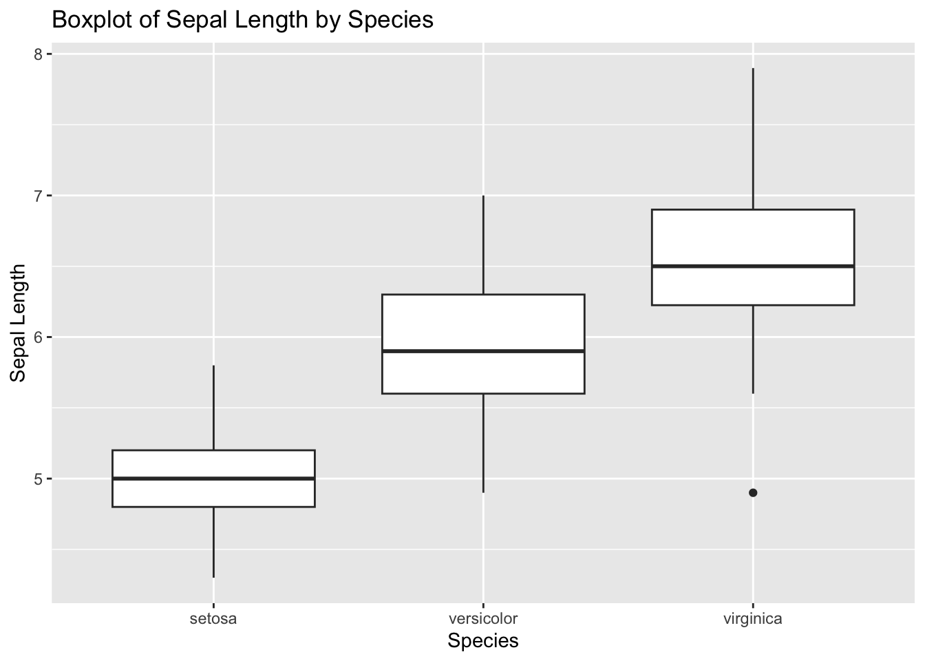
5. Create a Boxplot
Use ggplot2 to create a boxplot of Sepal_Length for each species.
ggplot (data = iris, aes (x = Species, y = Sepal.Length)) + geom_boxplot () + labs (title = "Boxplot of Sepal Length by Species" ,x = "Species" ,y = "Sepal Length" )
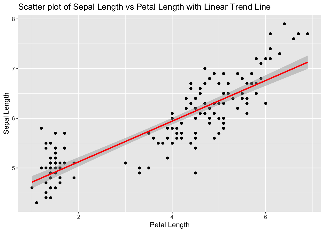
6. Create a Scatter Plot with Linear Trend Line
Use ggplot2 to create a scatter plot of Sepal_Length vs Petal_Length and add a linear trend line.
ggplot (data = iris, aes (x = Petal.Length, y = Sepal.Length)) + geom_point () + geom_smooth (method = "lm" , col = "red" ) + labs (title = "Scatter plot of Sepal Length vs Petal Length with Linear Trend Line" ,x = "Petal Length" ,y = "Sepal Length" )
`geom_smooth()` using formula = 'y ~ x'
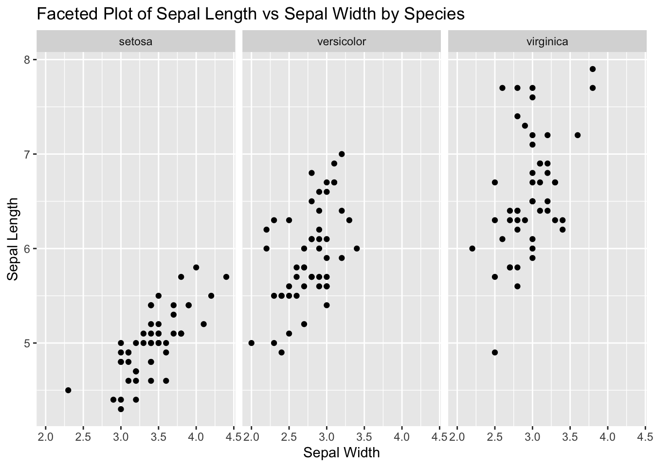
7. Create a Faceted Plot
Use ggplot2 to create a faceted plot of Sepal_Length vs Sepal.Width, faceted by Species.
ggplot (data = iris, aes (x = Sepal.Width, y = Sepal.Length)) + geom_point () + facet_wrap (~ Species) + labs (title = "Faceted Plot of Sepal Length vs Sepal Width by Species" ,x = "Sepal Width" ,y = "Sepal Length" )
Step 4: Combining Everything
Combine all steps into a single script to practice the workflow from data manipulation to visualization.
library (tidyverse)# Load dataset data (iris)# Data manipulation <- iris %>% select (Sepal_Length = Sepal.Length, Sepal.Width, Petal.Length, Petal.Width, Species)<- iris_selected %>% mutate (Sepal_Ratio = Sepal_Length / Sepal.Width, Petal_Ratio = Petal.Length / Petal.Width)<- iris_mutated %>% filter (Species == "setosa" ) %>% arrange (desc (Sepal_Length))<- iris_mutated %>% group_by (Species) %>% summarize (avg_Sepal_Length = mean (Sepal_Length), avg_Petal_Length = mean (Petal.Length))# Data visualization # Boxplot ggplot (data = iris, aes (x = Species, y = Sepal.Length)) + geom_boxplot () + labs (title = "Boxplot of Sepal Length by Species" ,x = "Species" ,y = "Sepal Length" )# Scatter plot with trend line ggplot (data = iris, aes (x = Petal.Length, y = Sepal.Length)) + geom_point () + geom_smooth (method = "lm" , col = "red" ) + labs (title = "Scatter plot of Sepal Length vs Petal Length with Linear Trend Line" ,x = "Petal Length" ,y = "Sepal Length" )# Faceted plot ggplot (data = iris, aes (x = Sepal.Width, y = Sepal.Length)) + geom_point () + facet_wrap (~ Species) + labs (title = "Faceted Plot of Sepal Length vs Sepal Width by Species" ,x = "Sepal Width" ,y = "Sepal Length" )